VLOOKUP in Microsoft Excel

If you need to translate a column value to another sheet vlookup is the function that will do the job.
In the next example I have one sheet with names and country codes, I need to show in this sheet instead of the country code the name of the country that is in another sheet.

This is my User sheet:

This is my Country codes sheet, The ID column (Country Code) has to be first:

To do the job follow the next steps:
Click on the User >> C2 field, this is the column where we are going to insert the country names
From the Excel Ribbon select Lookup & Reference >> VLOOKUP, a formula window will be showed

For the "Lookup_value" click on the field value that is going to join both sheets, in this case click on Country Code >> 1

For the "Table_Array" value, we need to select from the country reference sheet all the values where we are going to find the values, in this case I selected all the Country Code and Name columns

For the "Col_index_num" we need to indicate the column number of the information we need, in this case is column two from the Country sheet

To finish with this formula window we indicate the "Range_Lookup" there are two possible vales:

• FALSE if you need an exact match
• TRUE to find the closest match

Now press "OK" the window will be closed and you will have your formula as showed below:

If you copy ans paste the formula like this in the rest of the cells it will show the same value, to fix this and get the right value you need to modify the formula a little bit.
To fix the current formula:
                                       =VLOOKUP(B3,Country!A1:B4,2,FALSE)
Add the $ before the range of the "Table_Array" value, as showed below:
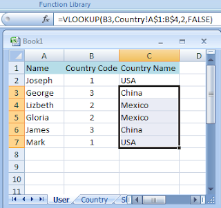
                                      =VLOOKUP(B3,Country!A$1:B$4,2,FALSE)

Now you can copy the formula in the rest of the fields, the result is showed below: